Saturday, September 28, 2019

Recursive Neural Networks

A Recursive Neural Network

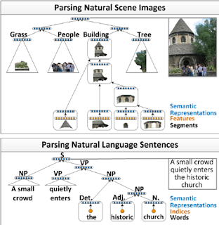
Recursively Neural Networks can learn to structure data such as text or images hierarchically. The network can be seen to work similar to a context free grammar and the output is a parse t
The figure below (from this paper) shows examples of parse trees for an image (top) and a sentence (bottom).


A recursive neural network for sequences always merges two consecutive input vectors and predicts if these two vectors can be merged. If so, we replace the two vectors with best merging score with the hidden vector responsible for the prediction. If done in a recursive manner, we can construct a parse tree.

Formally we can construct the network as follows. Given an input sequence $x = x_1 ... x_T, x_i \in \mathbb{R}^D$ then for two neighboring inputs $x_t, x_{t + 1}$ we predict a hidden representation:

$h_t  = \sigma(x_t W_l + b_l)$
$h_{t + 1} = \sigma(x_{t + 1} W_r + b_r)$

The hidden layer used for replacement is computed from the concatenation of the two previous hidden layers: $h=\sigma([h_t, h_{t + 1}] W_h + b_h)$. Finally, the prediction is simply another layer predicting the merging score.

For the implementation we define the neural network with the merging decision first. Given a node with the parent representations (for leaf nodes that are the input vectors) we build the hidden representations and then compute the merging score.
class NeuralGrammar(nn.Module):
    '''
    Given a tree node we project the left child and right child into
    a feature space cl and cr. The concatenated [cl, cr] is projected
    into the representation of that node. Furthermore, we predict
    the label from the hidden representation.
    '''

    def __init__(self):
        super(NeuralGrammar, self).__init__()
        self.left       = nn.Linear(IN, H, bias=True)
        self.right      = nn.Linear(IN, H, bias=True)
        self.parent     = nn.Linear(2 * H, IN, bias=True)
        self.projection = nn.Linear(IN, 1, bias=True) 

    def forward(self, node):        
        l = node.left_child.representation
        r = node.right_child.representation
        y = node.label
        x = torch.cat([torch.relu(self.left(l)), torch.relu(self.right(r))], 0)
        p = torch.tanh(self.parent(x))
        score = self.projection(p)
        return (p, score) 

Now we can implement our node class which also handles the parsing, by greedily merging up to a tree. A node in the tree holds it's representation as well as a left and a right child. In other words, each node represents a merging decision with the two children being the nodes merged and the parent representation being the hidden layer in the merger grammar. Parsing a tree involves merging the vectors with the highest score and replacing the nodes with their parent node.
    
class TreeNode:
    '''
    A tree node in a neural grammar. 
    Represented as a binary tree. Each node is also represented by
    an embedding vector.
    '''

    def __init__(self, representation=None):
        self.representation = representation
        self.left_child     = None
        self.right_child    = None

    def greedy_tree(cls, x, grammar):
        '''
        Greedily merges bottom up using a feature extractor and grammar
        '''
        T, D   = x.shape
        leafs  = [cls(x[i, :]) for i in range(T)] 
        while len(leafs) >= 2:
            max_score       = float('-inf')
            max_hypothesis  = None 
            max_idx         = None 
            for i in range(1, len(leafs)):
                # difference of reconstruction of the center of the span of the subtree in the spectrogram is the score
                # inspired by continuous bag of words
                hypothesis = cls(leafs[i - 1].start, leafs[i].stop)
                hypothesis.left_child     = leafs[i - 1]
                hypothesis.right_child    = leafs[i]
                representation, score     = grammar(hypothesis)
                hypothesis.representation = representation
                if score > max_score:
                    max_score      = score
                    max_hypothesis = hypothesis
                    max_idx        = i    
            leafs[max_idx - 1:max_idx + 1] = [max_hypothesis]            
        return leafs[0]
    
During learning, we collect the scores of the subtrees and use labels to decide if a merge was correct or not.
Thursday, August 1, 2019

Code Along Books: Bitcoin, Go Game, Ray Tracers

A scene rendered with your own ray tracer


I like learning by doing. In my opinion the only real self test whether you understood something is a working prototype. For example, when learning more about the details of deep learning or xgboost, I implemented my own auto differentiation and gradient boosted trees.

Recently I found several books that guide you through implementations of fairly complex pieces of software. After finishing a chapter it feels like making progress on a project. So it is easier to follow along and you don't have to search for all the references needed yourself. You still have the benefit from learning by doing.

The book based projects I found are: 
  1. A ray tracer [1]
  2. A go AI [2]
  3. A bitcoin implementation [3]
  4. A Prolog interpreter [4]
The prolog interpreter needed a little more adjustment since the book's topic is classic
AI in lisp and I wanted to implement my prolog in scala.

The previous projects on neural networks were based on Goodfellow's Deep Learning book [5] and many other references such as online classes so it was not as easy to code along. The same is true for the gradient boosting implementation which was mostly based on papers and books.

However the other projects simply involved writing code and the book was the only thing required to get into the topic. The quality all of these books show is that it is not a collection of separated code pieces that explain a topic but the topic's are explained by a coherent code based that you develop yourself form scratch.

1. A Ray Tracer

The book "The Ray Tracer Challenge: A Test Driven Guide to Your First 3D Rendered" [1], is giving you no actual code but behavior specifications (cucumber). The code has to be written by yourself.
Harder parts include pseudo code. The book covers the basic math library and then uses the defined primitives to construct more and more complex features.
The end result is a full ray tracer with shadows reflections and multiple primitives.

2. A Go AI

In the next book: "Deep Learning And The Game Of Go" [2], you build a go AI using the code provided by the authors. The books walks you through the implementation of the go board and rules first. Then the authors walk through classic game AI algorithms such as monte carlo tree search. In the end the authors introduce game state evaluation using convolutional neural networks using Keras.
The resulting system resembles an early version of AlphaGO


3. Bitcoin

The book "Programming Bitcoin" [3] is a mix between the first two. Lot's of code is provided in the form of skeletons but the reader still has to fill in the blanks for several assignments. The book
covers everything from basic cryptography to scripting bitcoin. The end result is a full bitcoin 
implementation.


Wrap up

The great thing about all the books mentioned is that all these books do cover the primitives needed too. You don't need to rely on a library but the authors walk you front to back.

My code bases are all on github. Some are work in progress [WIP] since
i did not finish the books yet. For example, in books 2 and 3 I only went through the first chapters:


  1. The ray tracer
  2. The go AI
  3. The bitcoin implementation
  4. The Prolog interpreter

REFERENCES:


[1] Buck, "The Ray Tracer Challenge: A Test Driven Guide to Your First 3D Rendered", Pragmatic Bookshelf, 2019
[2] Pumperla, Furguson, "Deep Learning And The Game Of Go", Manning, 2019
[3] Song, "Programming Bitcoin: Learn How To Program Bitcoin From Scratch", Oreilly, 2019
[4] Norvig: "Paradigmes of Artificial Intelligence Programming: Case Studies in Lisp", Morgan Kaufmann, 1992
[5] Ian Goodfellow, "Deep Learning", MIT Press, 2016

Tuesday, July 9, 2019

WebRTC and Tensorflow.js

WebCam image classification on web page


I will give a quick tutorial on how to connect a webcam in html5/WebRTC to Tensorflow.js for image classification. We will load a pre trained mobile net and then pass it frames from the camera. First, we define our html page and specify a video element in which we later stream the video from the camera,
a label field and also start the WebRtc + neural network code. The code can be found at this gist.


<!DOCTYPE html>
<html>
  <head>
    <title> Hello WebRTC </title>
    <script src="https://cdn.jsdelivr.net/npm/@tensorflow/tfjs@1.0.0/dist/tf.min.js"></script>
  </head>
  <body>
    <video id="cam" width="224" height="224" autoplay playsinline></video> <br/>
    <script src="camnet.js"></script><br/>
    <font color="red" size="5"> LABEL: </font><br/>
    <div id="label"> </div>
  </body>
</html>


Then we download the pretrained mobile net and initialize the webcam.
 async function init() {
    try {
 const net = await tf.loadLayersModel(MOBILENET_MODEL_PATH);
        const constraints = window.constraints = {audio: false, video: true};
     const stream = await navigator.mediaDevices.getUserMedia(constraints);
     onSuccess(stream, net);
    } catch (e) {
     onError(e);
    }
}


The camera stream can be retrieved by the getUserMedia function. The onError method simply writes an error to the console. If we are successful, we get the video element from our dom and bind the stream to the video. We then start the detection loop with a method called onFrame.
function onSuccess(stream, net) {    
    const video = document.querySelector('video');
    const videoTracks = stream.getVideoTracks();
    console.log('Got stream with constraints:', constraints);
    console.log(`Using video device: ${videoTracks[0].label}`);
    window.stream = stream;
    video.srcObject = window.stream;
    onFrame(video, net);
}


onFrame's inner function processFrame is an infinite recursion. We grab the video frame by frame and push it into a classify method along with the neural network, the video element as well as the label element.
function onFrame(video, net) {
    var label_element = document.getElementById('label');
    console.log(net.summary());
    async function processFrame() {
 classify(video, label_element, net)
        requestAnimationFrame(processFrame);          
    }
    processFrame();
}
The last method transforms the camera image into a tensor, normalizes the color and then construct a batch with only one example. Based on the prediction from the mobile net, we extract the best class and write it into the label element.
async function classify(img_element, label_element, net) {
    const img = tf.browser.fromPixels(img_element).toFloat();
    const offset = tf.scalar(127.5);
    const normalized = img.sub(offset).div(offset);
    const batched = normalized.reshape([1, IMAGE_SIZE, IMAGE_SIZE, 3]);
    const prediction = await net.predict(batched).data();
    var max_i = 0;
    var max_v = prediction[0];
    for (let i = 0; i < prediction.length; i++) {
 if(prediction[i] > max_v) {
     max_v = prediction[i];
     max_i = i;
 }
    }
    const label = IMAGENET_CLASSES[max_i];
    if (max_v > 0.5) {
 label_element.innerHTML = label + " [" + max_v + "]";
    }
}


Sunday, July 7, 2019

Implementing Triplet Loss Function in Tensorflow 2.0

In this post I will go through an implementation of the triplet loss for siamese neural network architectures in keras (tensorflow 2.0).

The goal of training a neural network with a triplet loss is to learn a metric embedding. That is examples that are conceptually close are also close in euclidean space and examples that are conceptually further are further away in euclidean space, too. The triplet loss is introduced in the facenet paper from google. When learning with the triplet loss, we choose three examples. The first example is called the anchor, which can be any example from our dataset. The positive example is one that is conceptually close. For example, a conceptually close example for face recognition might be a picture of the same person as shown in the anchor image. The negative example might simply be a picture of any other person. The embedding network can actually have any architecture. During training, we push all three examples through the network, compute the loss function with the three embeddings and adjust the weights which in each epoch pushes negative examples further from it's anchors and positive examples closer.


Figure 1: The Triplet loss forces negative examples further from the anchor and positive examples closer. 
An example is shown below. The loss consists of three parts. The first is the euclidean distance between the anchor and it's positive example. The second is the euclidean distance between the anchor and it's negative example. Since we want to minimize the loss, the first term should be small and the second term should be large. Furthermore, we introduce a regularization term or margin between the examples.

Figure 2: We embed the anchor, positive and negative examples with the same network and apply the triplet loss. During Backpropagation we achieve higher euclidean distances to the negative example and lower distances for the negative examples. 


For unsupervised audio embedding, one way to sample triplets is to pick a window from the audio as the anchor and a close window in time to the anchor as positive (since audio does not change that rapidly). The negative example is simply a sample from another file.

In order to implement such a loss in  Tensorflow 2.0 / Keras, we can implement the Loss base class.

class TripletLoss(loss.Loss):

    def __init__(self, margin):
        super().__init__()
        self.margin = margin

    def call(self, y_true, y_pred):
        anchor = y_pred[0]
        pos    = y_pred[1]
        neg    = y_pred[2]
        pos_dist   = tf.reduce_sum(tf.square(tf.subtract(anchor, pos)), axis=-1)    
        neg_dist   = tf.reduce_sum(tf.square(tf.subtract(anchor, neg)), axis=-1)    
        basic_loss = tf.add(tf.subtract(pos_dist, neg_dist), self.margin)    
        loss       = tf.reduce_sum(tf.maximum(basic_loss, 0.0))               
        return loss

As you can see from the code, we do not need the ground truth (y truth) and we simply pass dummy values during training (Keras will still check it's dimension). In order to construct a model using the triplet loss, we can build an embedder model and then use that model three times in the triplet loss model. During back propagation, the three gradients will be summed and then passed through the embedder model (deep learning book chapter 6, Algorithm 6.6). In order to see a full example for
audio data, you can check this gist.


Monday, April 1, 2019

Navigable Small World Graphs for Approximate Nearest Neighbors: Implementation in Rust and Time Series Experiments.

A navigable small world graph. Image from NSWG

A small world graph or network, is a mathematical graph with certain properties. In such a graph most nodes will not be neighbors but two neighbors of a node will likely be. In other words, traversing the graph from one node to the other can be achieved in very few edge transitions.
The idea is to use such a structure to support fast approximate nearest neighbor queries.
In a navigable small world graph (NSWG) each node or vertex is associated with a vector in $\mathbb{R}^d$. During search, we check the distance to all neighbors of the node and transition to the closest one. We then repeat the search until we found a local minimum. In this post we discuss how to compute the $k$ closest neighbors and explore the method using the UCR time series
dataset. The code can be found on github.

Modelling the Graph and Search Results

The edges in the graph are implemented using a map. For each vertex, we map to the neighboring vertices. The struct also holds the flattened vectors associated with each vertex.
/// A navigable small world graph defined
/// by a sparse edge set and a flat vector set, one for each vertex.
pub struct NavigableSmallWorldGraph {
    pub edges: HashMap<usize, Vec<usize>>,
    pub instances: Vec<f32>,
    pub dim: usize
}
A search result is simply implemented as a struct with a node id as well as a distance to the query.
pub struct SearchResult {
    pub node: usize,
    pub distance: f32
}

Furthermore, we implement comparing to search results by their distance. In order to manage the set of candidates during knn search, we implement a result set as a bineary tree set. In this way, extracting the top neighbors is fast.
pub struct ResultStore {
    ordered: BTreeSet<SearchResult>
}

impl ResultStore {    

    pub fn new() -> ResultStore {
        ResultStore { ordered: BTreeSet::new() }
    }

    pub fn len(&self) -> usize {
        self.ordered.len()
    }

    pub fn take(&self, k: usize) -> Vec<SearchResult> {
        self.ordered.iter().take(k).map(|x| x.clone()).collect()
    }

    pub fn best(&self, at: usize) -> SearchResult {
        let k_best = self.ordered.iter().take(at);
        if k_best.len() < at {
            SearchResult::none()
        } else {
            k_best.last().unwrap().clone()
        }
    }

    pub fn insert(&mut self, result: SearchResult) {
        self.ordered.insert(result);
    }
    
    pub fn remove(&mut self, result: &SearchResult) {
        self.ordered.remove(result);
    }

}
Insertion in this data structure automatically inserts in order. The same goes for the remove option, which keeps the tree ordered. Iterating the elements now allows to get the candidates sorted.

KNN-Search and Graph Construction

First we define the distances we support. For this post, I implement the euclidean distance between a query vector and a node in the graph as well as the dynamic time warping distance, when seeing the vectors as time series. If we give a warping band to the distance function, we compute the dtw distance.
    fn distance(&self, query: &[f32], node: usize, align_band: Option) -> f32 {
        match align_band {
            Some(w) => self.dtw(query, node, w),
            None    => self.euclidean(query, node)
        }
    }

    fn euclidean(&self, query: &[f32], node: usize) -> f32 {
        assert!(query.len() == self.dim);
        let y = &self.instances[node  * self.dim .. (node + 1) * self.dim];
        let mut distance = 0.0;
        for i in 0 .. query.len() {
            distance += f32::powf(query[i] - y[i], 2.0);
        }
        f32::sqrt(distance)
    }

    fn dtw(&self, query: &[f32], node: usize, w: usize) -> f32 {
        let y  = &self.instances[node  * self.dim .. (node + 1) * self.dim];
        let n  = query.len();
        let m  = y.len();
        // allocating here is the main bottleneck
        let mut dp = vec![std::f32::INFINITY; (n + 1) * (m + 1)]; 
        dp[0] = 0.0;
        for i in 1 .. n + 1 {
            for j in usize::max(NavigableSmallWorldGraph::sub(i, w), 1) .. usize::min(i + w, m + 1) {
                let distance = f32::powf(query[i - 1] - y[j - 1], 2.0);                
                dp[i * (n + 1) + j] = distance + NavigableSmallWorldGraph::min3(
                    dp[(i - 1) * (n + 1) + j],
                    dp[i       * (n + 1) + (j - 1)], 
                    dp[(i - 1) * (n + 1) + (j - 1)]
                )
            }
        }
        dp[dp.len() - 1]
    }
We can now turn to the search algorithm. During the search, we maintain an ordered candidate lost, an ordered result list and an unordered visited set. During a search run, we start with a random entry node. We then add said node as the first candidate. In the following steps, we get the best node from the candidate list and add all of it's neighbors as candidates, as long as we did not visit the node before. If a candidate is further away then the k-th neighbor so far, we stop. We restart the search $n$ times from different random start points.
    /// Given a query find the k-nearest neighbors using the nswg graph
    /// * `query` The query vector
    /// * `n_searches` number of restarts
    /// * `k_neighbors` number of results
    /// * `align_band` Sakoe Chiba Band for Dynamic Time Warping, if not set we use Euclidean Distance
    pub fn search(
        &self,
        query: &[f32],
        n_searches: usize,
        k_neighbors: usize,
        align_band: Option<usize>,
    ) -> (Vec<SearchResult>, usize) {
        let mut candidates = ResultStore::new();
        let mut results = ResultStore::new();
        let mut visited = HashSet::new();
        let mut rng = rand::thread_rng();
        let mut n_steps = 0;
        for _attempt in 0..n_searches {
            let mut bsf = ResultStore::new();
            // stop if we visited all of the nodes
            if self.n_instances() == visited.len() {
                break;
            }
            // sample entry point, make sure we never used it before
            // and insert the point as a candidate
            let mut entry_point = rng.gen_range(0, self.n_instances());
            while visited.contains(&entry_point) {
                entry_point = rng.gen_range(0, self.n_instances());
            }
            let distance = self.distance(query, entry_point, align_band);
            candidates.insert(SearchResult::new(entry_point, distance));
            while candidates.len() > 0 {
                // check if we can stop: abendon search if the result is the worst than the top k so far
                let candidate = candidates.best(1);
                let kth = f32::min(
                    results.best(k_neighbors).distance,
                    bsf.best(k_neighbors).distance,
                );
                candidates.remove(&candidate);
                if candidate.distance > kth {
                    break;
                }
                // add expand all edges
                for edge in self.edges[&candidate.node].iter() {
                    if !visited.contains(edge) {
                        n_steps += 1;
                        visited.insert(edge);
                        let edge = *edge;
                        let distance = self.distance(query, edge, align_band);
                        candidates.insert(SearchResult::new(edge, distance));
                        bsf.insert(SearchResult::new(edge, distance));
                    }
                }
            }
            for res in bsf.take(k_neighbors) {
                results.insert(res);
            }
        }
        (results.take(k_neighbors), n_steps)
    }

Testing the Code on UCR Time Series

In order to test the code, we run it against multiple datasets from the UCR time series archive. Our accuracy is similar to the UCR datasets. However, the number of distance computations is way less.

Saturday, March 16, 2019

Avro Rust: A first look at data serialisation in rust using avro

Avro is a data serialisation system in which you can define a schema (basically the fields in a record you want to serialise along with their type) in json and then send the data binary.


In the Rust language, structs can be serialised to multiple formats using a library called serde. In the
last post  we saved our word2vec model into a binary format using serde and bincode. In this post, we will look into serialising with serde and avro-rs, an avro implementation in rust and implement sending serialised objects over a tcp stream using framing.

As usual the code is on [:github:]


Data (De) Serialisation 

Avro supports several data types for serialisation including more complex types such as arrays.


 #[derive(Debug, Deserialize, Serialize)]
pub struct Test {
    a: i32,
    b: f64,
    c: String,
    d: Vec<i32>
}

fn schema() -> Schema {
    let raw_schema = r#"
            {
                "type": "record",
                "name": "test",
                "fields": [
                    {"name": "a", "type": "int",    "default": 0},
                    {"name": "b", "type": "double", "default": 1.0},
                    {"name": "c", "type": "string", "default": "dansen"},
                    {"name": "d", "type": {"type": "array", "items": "int"}}
                ]
            }
        "#;
    avro_rs::Schema::parse_str(raw_schema).unwrap()
}

In the code above, we define a struct that we want to serialise and define the serialisation schema in json. Nothing more is needed. With this information we can serialise and deserialise the `Test` struct. We can even (de) serialise a collection of these structs. The serialisation results in a vector of bytes and given this vector of bytes we can deserialise into a vector of our original struct.
 #[derive(Debug, Deserialize, Serialize)]
fn write_data(data: &[Test], schema: Schema) -> Vec<u8> {
    let mut writer = Writer::with_codec(&schema, Vec::new(), Codec::Deflate);
    for x in data.iter() {
        writer.append_ser(x).unwrap();
    }
    writer.flush().unwrap();
    writer.into_inner()
}

fn read_data(data: &[u8], schema: Schema) -> Vec<Test> {
    let reader = Reader::with_schema(&schema, data).unwrap();
    reader
        .map(|record| from_value::<Test>(&record.unwrap()).unwrap())
        .collect()
}

Framed Writing and Reading over TCP/IP

In order to send avro over the network, it seems recommended to frame the message. That means breaking our byte stream into chunks we send over, each preceded by it's length and terminated by a 0 sized chunk. Avro messages are framed as a list of buffers. Framing is a layer between messages and the transport. It exists to optimize certain operations. The format of framed message data is: a series of buffers, where each buffer consists of: a four-byte, big-endian buffer length, followed by that many bytes of buffer data. A message is always terminated by a zero-length buffer. Framing is transparent to request and response message formats (described below). Any message may be presented as a single or multiple buffers. Framing can permit readers to more efficiently get different buffers from different sources and for writers to more efficiently store different buffers to different destinations. In particular, it can reduce the number of times large binary objects are copied. For example, if an RPC parameter consists of a megabyte of file data, that data can be copied directly to a socket from a file descriptor, and, on the other end, it could be written directly to a file descriptor, never entering user space. A simple, recommended, framing policy is for writers to create a new segment whenever a single binary object is written that is larger than a normal output buffer. Small objects are then appended in buffers, while larger objects are written as their own buffers. When a reader then tries to read a large object the runtime can hand it an entire buffer directly, without having to copy it. from Avro Page .

Writing over the network with a fixed buffer or chunk size can be implemented by sending slices of the given size over the network, each preceded by the length of it (which really only matters for the last one). As described above we send the size of the buffer as a 4-byte integer, big endian.


 pub fn send_framed(objects: &[Test], address: String, schema: Schema, buf_size: usize) {
    let data = write_data(objects, schema);
    let mut stream = TcpStream::connect(address).unwrap();
    let n = data.len();
    for i in (0..n).step_by(buf_size) {
        // determine size of bytes to write
        let start = i;
        let stop = usize::min(i + buf_size, n);
        // send length of buffer
        let mut buffer_length = [0; 4];
        BigEndian::write_u32(&mut buffer_length, (stop - start) as u32);
        stream.write(&buffer_length).unwrap();
        // write actual data
        stream.write(&data[start..stop]).unwrap();
    }
    // terminate by 0 sized
    let mut buffer_length = [0; 4];
    BigEndian::write_u32(&mut buffer_length, 0);
    stream.write(&buffer_length).unwrap();
    stream.flush().unwrap();
}


When reading we simply read the size of the next buffer, then read it and append it into a vector of bytes until we hit the zero size buffer marking the end. Then we simply use the method above to de serialise into a vector of structs
 
pub fn read_framed(stream: &mut TcpStream, schema: Schema) -> Vec<Test> {
    let mut message: Vec<u8> = Vec::new();
    let mut first_buf = [0; 4];
    stream.read(&mut first_buf).unwrap();
    let mut next = BigEndian::read_u32(&first_buf);
    // read while we see non empty buffers
    while next > 0 {
        // append all bytes to final object
        let mut object = vec![0; next as usize];
        stream.read(&mut object).unwrap();
        message.append(&mut object);
        // read next buffer size
        let mut next_buf = [0; 4];
        stream.read(&mut next_buf).unwrap();
        next = BigEndian::read_u32(&next_buf);
    }
    read_data(&message, schema)
}


Thats it, now we can send avro framed over the network and de-serialise on the other end.

Friday, March 8, 2019

Word2Vec Implementation in Rust: Continuous Bag of Words


I recently started to get serious about learning rust and I needed a small to medium project to train on.
One thing I explained in this blog and walked through the code is Word2Vec. A method to learn word embeddings. In this post I will explain the method again using my new rust code on github.

Word Similarity - Basic Idea 

In the following, I will describe the basic idea behind continuous bag of words, one way to estimate word vectors. Word vectors are a dense vectorised word representation capturing similarity of words in Euclidean space. Basically we have one vector for each word in our vocabulary. The euclidean distance between two vectors of words that are similar is smaller than the distance between vectors of words that are less similar. The assumption in Word2Vec is that words that appear in a similar context are similar. We shift a sliding window over the text and try to predict the center word in the window from the word vectors of the surrounding words in the window. 

pub struct Window<'a> {
    pub words:       &'a [usize], 
    pub predict_pos: usize
}

pub struct Document {
    pub words: Vec<usize>
}

impl<'a> Window<'a> {

    pub fn label(&self) -> usize {
        self.words[self.predict_pos]
    }

}

impl Document {

    pub fn window(&self, pos: usize, size: usize) -> Option<Window> {
        let start = sub(pos, size);
        let stop  = usize::min(pos + size, self.words.len() - 1); 
        if stop - start == 2 * size {
            Some(Window {words: &self.words[start as usize .. stop as usize], predict_pos: size})
        } else {
            None
        }
    }

}

The code above defines a document as a vector of word ids and allows to shift a sliding window over it. The return type is not a vector itself but a slice, which is convenient since there is nothing copied. In the following the center word in the window is called a label $l$ and the other words are called the context: $c_1 .. c_m$.

Word Vectors

Now that we have defined the window, we can start implementing a representation for the word vectors. There will be one vector of $d$ dimensions or columns per word in the dictionary.
In code we save the word vectors as a flat vector of doubles. We can then access the $i-th$ vector as a slice from $[i * cols .. (i + 1) * cols]$


#[derive(Serialize, Deserialize)]
pub struct ParameterStore {
    pub cols: usize,
    pub weights: Vec<f64>
}

impl ParameterStore {

    pub fn seeded(rows: usize, cols: usize) -> ParameterStore {
        let mut rng = rand::thread_rng();
        let mut weights = Vec::new();
        for _i in 0 .. (rows * cols) {
            let uniform = (rng.gen_range(0.0, 1.0) - 0.5) / cols as f64;
            weights.push(uniform);
        }
        ParameterStore {cols: cols, weights: weights}
    }

    pub fn at(&self, i: usize) -> &[f64] {
        let from = i * self.cols;
        let to = (i + 1) * self.cols;
        &self.weights[from .. to]
    }

    pub fn update(&mut self, i: usize, v: &Vec<f64>) {
        let from = i * self.cols;
        for i in 0 .. self.cols {
            self.weights[i + from] += v[i];
        }
    }

    pub fn avg(&self, result: &mut Vec<f64>, indices: Vec<usize>) {
        for col in 0 .. self.cols {
            result[col] = 0.0;
            for row in indices.iter() {
                let from = row * self.cols;
                result[col] += self.weights[col + from];
            }
            result[col] /= indices.len() as f64;
        }
    }

}


We initialise the vectors by a random number in the range $\frac{Uniform([-0.5;0.5])}{d}$, which is the standard way to initialise word2vec.  The update method simply adds a gradient to a word vector. There is also a method to compute the average of multiple word vectors, needed later during learning.

Putting It All Together: Computing the Gradients

So now we can compute windows from the text and average the word vectors of the context words. 
The averaged vectors are our hidden layer's activations. From there we compute the prediction and then back propagate the error. So we need two sets of parameters. One is the word vectors initialised as above, and one for the predictions which is initialised to zeros. 

#[derive(Serialize, Deserialize)]
pub struct CBOW {
    pub embed:   ParameterStore,
    pub predict: ParameterStore
}

Given the average embedding for the context as $h$ and the vector for word $i$ from the predictions $w_i$, the forward pass on the neural network is:

$a_i = \sigma(h * w_i)$.

We are predicting the center word of the window, that means we model the output layer as a multinomial where the center word is one hotcoded. So output should be $1$ for the center word
and $0$ for all others. Then the error for the center word is:

$e_i = log(a_i) $

and for all others it is

$e_i = log(1 - a_i)$.

The gradient on the loss is simply $\delta_i = (y - a_i) * \lambda$, with $\lambda$ being the learning rate.

 fn gradient(&self, label: usize, h: &Vecf&lt64>, truth: f64, rate: f64) -> (f64, f64) {        
        let w = self.predict.at(label);
        let a = sigmoid(dot(&h, &w));
        let d = (truth - a) * rate;
        let e = -f64::ln(if truth == 1.0 {a} else {1.0 - a});    
        (d, e)
    } 

The gradient applied to the output parameters is: $\delta_i * h$. The gradient for the embeddings is: $\delta_i * w_i$ which is applied to all context words. So all words in the same context are updated with the same gradient, in turn making them more similar, which was the main goal for word embeddings. There is one more detail. Normally, we would have to compute the losses for the complete dictionary, however for a million words, that would take very long. So instead we use something called negative sampling. We compute the gradient for the center word and then sample some negative words as the negative gradient.
The final computation for learning is shown below:
 pub fn negative_sampeling(&mut self, window: &Window, rate: f64, n_samples: usize, unigrams: &Sampler) -> f64 {
        let mut gradient_embed = vec![0.0; self.embed.cols];
        let h = self.embedding(self.ids(window));        
        let (pos, pos_err) = self.gradient(window.label(), &h, 1.0, rate);        
        let mut error = pos_err;
        let mut gradient_pos_predict = vec![0.0; self.predict.cols];
        for i in 0 .. self.embed.cols {        
            gradient_embed[i] += pos * self.predict.at(window.label())[i];
            gradient_pos_predict[i] += pos * h[i];
        }
        self.predict.update(window.label(), &gradient_pos_predict);
        for _sample in 0 .. n_samples {
            let token = unigrams.multinomial();
            let (neg, neg_error) = self.gradient(token, &h, 0.0, rate);
            error += neg_error;
            let mut gradient_neg_predict = vec![0.0; self.predict.cols];
            for i in 0 .. self.embed.cols {
                gradient_embed[i]       += neg * self.predict.at(token)[i];
                gradient_neg_predict[i] += neg * h[i];
            }
            self.predict.update(token, &gradient_neg_predict);
        }
        let ids = self.ids(window);
        for i in 0 .. ids.len() {
            self.embed.update(ids[i], &gradient_embed);
        }
        error
    }

Results

I trained the net on quora questions and when searching for similar vectors we will find similar words:

Searching: India
kashmir: 11.636631273392045
singapore: 12.155846288647625
kerala: 12.31677547739736
dubai: 12.597659271137639
syria: 12.630908898646624
pradesh: 12.657158343619573
pok: 12.667834993874745
malaysia: 12.708228117809442
taiwan: 12.75190112716203
afghanistan: 12.772290465531222
africa: 12.772372266369985
bjp: 12.802207718902666
karnataka: 12.817502941769622
europe: 12.825095372204384

Thursday, January 10, 2019

Scala3D: Implementing A Wolfenstein Like Ray Casting Engine

Introduction

I recently got interested in 3D game engines for realistic images. I am currently reading through
a book describing a complete ray tracing algorithm [3]. However, since there is a lot of coding to do and a lot of complex geometry, I searched for a simpler side project. I then started to look into 2D
ray casting to generate 3D environments, as used in the Wolfenstein 3D engine. There are several
descriptions on how to build one [1,2]. However, the Wolfenstein black book [1] talks a lot about memory optimisations and execution speed. Lots of the chapters include assembly code and c snippets dealing with the old hardware. Implementing something like this is way easier, now.
Computers got way faster and programming languages way more convenient. So I decided to
build a clone in Scala. The result can be seen in the video above. The left side is the 3D view, and the right side shows a 2D map view. The red lines are the rays from the ray casting algorithm which represent what the player sees and the green line is the camera. The code can be found here [:github:]. If you want to move in the map use "WASD".

Assumptions About The World

The world in Wolfenstein 3D is represented by a flat grid. Different heights in the map are not possible. All objects stand on the same plane and have to be boxes. This assumption makes a lot of things easier. In a 3D engine, the main task is to determine what is seen from a specific view (the player's camera). The nice thing is that we do not have to determine what is visible in any possible direction, because we are moving on a plane, which restricts us to a 2D problem. The second assumption of a world on a grid will simplify the calculation of ray to box intersection later.

Implementing The Player And Camera

The basic idea is to describe a player in 2D by it's position: $p = (p_x, p_y)$. Furthermore, we save the position the player is looking at: $d = (d_x, d_y)$. We also save the image plane: $i = (i_x, i_y)$ which is perpendicular to the player.

In the image above the image plane is marked in green, and the rays for collision are marked in green. In order to calculate the direction for each ray, we first calculate the x coordinate in camera space as $c_x = 2 * x / w$ where $x$ is the row in the image and $w$ is the width of the image, then we compute the ray from the player that goes through that position as:
  • $r_{dx} = d_x + i_x * c_x$
  • $r_{dy} = d_y + i_y * c_x$
Now we can follow each ray until we hit a wall.

Digital Differential Analysis Ray Casting


In order to find what wall we see at the image row $c_x$, we follow the ray until it hits a wall. We initialize the search by calculating the distance to the first time the ray hits the x-axis (in the image this is the segment $a$ to $b$) and the first time we hit the y axis (in the image this is the segment $a$ to $c$). From there we estimate the slope $\delta = (\delta_x, \delta_y)$ in x and y which tells us how far we have to travel to hit each axis again. We then travel in the closest next grid position and check if the position is a wall hit.
    @tailrec
    private def traceRay(
        grid: Vector2D[Int], 
        sideDist: Vector2D[Double], 
        side: Int,
        deltaDist: Vector2D[Double],
        step: Vector2D[Int], 
        hit: Boolean,
    ): Hit = 
        if(hit) Hit(grid, side)
        else sideDist match {
            case Vector2D(x, y) if x < y => 
                traceRay(
                    Vector2D[Int](grid.x + step.x, grid.y),
                    Vector2D[Double](sideDist.x + deltaDist.x, sideDist.y),
                    0,
                    deltaDist,
                    step,
                    world.collids(grid.x + step.x, grid.y)
                )
            case Vector2D(x, y) if x >= y => 
                traceRay(
                    Vector2D[Int](grid.x, grid.y + step.y),
                    Vector2D[Double](sideDist.x, sideDist.y + deltaDist.y),
                    1,
                    deltaDist,
                    step,
                    world.collids(grid.x, grid.y + step.y)
                )
        }
In the implementation we move through the grid bu the delta distance and the current side distance (distance traveled along the $x$ and $y$ component). We also save which side ($x$ or $y$) we hit the wall at. In the recursion we follow the closest next map square until we find a hit and then return the position of the hit $h = (h_x, h_y)$ as well as the side.

Rendering A Scene


So for each image row, we run the ray tracer until we hit a wall. We then compute the distance to the wall in order to calculate how high the wall appears in the image $w_d$ from the player position, the hit position, the step size and the direction:
    private def projectedDistance(
        hit: Hit,
        pos: Vector2D[Double], 
        step: Vector2D[Int], 
        dir: Vector2D[Double], 
    ): Double = 
            if (hit.side == 0) (hit.pos.x - pos.x + (1 - step.x) / 2.0) / dir.x
            else               (hit.pos.y - pos.y + (1 - step.y) / 2.0) / dir.y
The height of the wall is then simply $l_h = \frac{h}{w_d}$. We then compress the slice of the texture we hit to that height and paint it in the image at the row position we send the ray for.

References

[1] GAME ENGINE BLACK BOOK: WOLFENSTEIN 3D, 2ND EDITION, 2018