Tuesday, November 6, 2018

Lindenmayer system: Implementation


I recently got interested in Lindenmayer systems or L-system for short and I also wrote some code.  These are generative 
systems that generate strings, that in turn can be interpreted as turtle graphics. For example, 
you can model koch curves and the famous dragon curve. This book describes how to generate plants which you can see below.


Implementation


For example, given a initial string $+A-Bf$, we have terminal symbols $\{+,-,f\}$ and non terminals $\{A, B\}$ that can still be replaced by rules like $A \rightarrow AfA$, which reads: each A can be replaced in the string. Furthermore, the string $+A-Bf$ can be interpreted by a turtle as $+$: turning right, $-$: turning left, all capital letters mean moving forward drawing a line, and all lower case letters mean moving silently to the next position. We start by defining a symbol class.
case class Symbol(id: Char) {

  def isSilent: Boolean = id.isLower

  def isTerminal: Boolean = !id.isLetter || id.isLower

}

Next we define a Lindenmayer system as a start string and a set of rules. Given the start string and a depth limit, we can recursively replace all non terminal symbols with the associated rules. This enables us to generate string.
case class LSystem(start: List[Symbol], rules: Map[Symbol, List[Symbol]]) {

  private def produce(symbol: Symbol): List[Symbol] =
    if(symbol.isTerminal) List(symbol)
    else rules(symbol)

  @tailrec
  private def produce(current: List[Symbol], result: List[Symbol]): List[Symbol] = current match {
    case Nil          => result
    case head :: tail => {
      produce(tail, result ::: produce(head))
    }
  }

  @tailrec
  private def produce(current: List[Symbol], stepsLeft: Int): List[Symbol] =
    if(stepsLeft == 0) current
    else produce(produce(current, Nil), stepsLeft - 1)

  def produce(depth: Int): List[Symbol] = produce(start, depth)

}
Now we are done with the definition of the grammar system. The only thing left is to define a turtle and an interpreter that converts strings from L-systems to a sequence of turtles. I define a turtle by it's posture $[x, y, \alpha]$ where $x,y$ is the turtle's position and the orientation is defined by the angle $\alpha$. For moving forward the next positions are defined as:
  • $x + \delta * cos(\alpha)$
  • $y + \delta * sin(\alpha)$
A rotation basically involves increasing the angle by some certain degree.
case class Turtle(x: Int, y: Int, angle: Double, sil: Boolean) {

  def move(distance: Int): Turtle =
    Turtle(
        math.round(x + distance * math.cos(math.toRadians(angle))).toInt, 
        math.round(y + distance * math.sin(math.toRadians(angle))).toInt, angle, false)

  def moveSil(distance: Int): Turtle =
    Turtle(
        math.round(x + distance * math.cos(math.toRadians(angle))).toInt, 
        math.round(y + distance * math.sin(math.toRadians(angle))).toInt, angle, true)

  def turn(by: Double): Turtle = {
    Turtle(x, y, (angle + by) % 360, false)
  }

  def silence: Turtle = Turtle(x, y, angle, true)
Then given a string, we can recursively build a sequence of positions by applying the action associated with each symbol.
class TurtleInterpreter(moveBy: Int, turnBy: Double) {

  import TurtleInterpreter._

  private def execute(cmd: List[Symbol], state: Turtle, stack: List[Turtle], drawable: List[Turtle]): List[Turtle] = cmd match {
    case Nil => drawable
    case RotateRight :: tail => execute(tail, state.turn(turnBy), stack, drawable)
    case RotateLeft  :: tail => execute(tail, state.turn(-turnBy), stack, drawable)
    case PushStack   :: tail => execute(tail, state, state :: stack, drawable)
    case PopStack    :: tail => execute(tail, stack.head.silence, stack.tail, stack.head.silence :: drawable)
    case head        :: tail => {
      val next = if (head.isSilent) state.moveSil(moveBy) else state.move(moveBy)
      execute(tail, next, stack, next :: drawable)
    }
  }

  def execute(cmd: List[Symbol], init: Turtle): List[Turtle] =
    execute(cmd, init, List.empty[Turtle], List(init))

}

object TurtleInterpreter {

  final val RotateRight = Symbol('+')
  final val RotateLeft  = Symbol('-')
  final val PushStack   = Symbol('[')
  final val PopStack    = Symbol(']')
Given that we can define grammars and paint pictures as the ones shown above. I wrote some code that plots all the above images that can be found on github.

Saturday, November 3, 2018

Exploring Super Resolution With Neural Networks: Blade Runner Style

In Blade Runner there is a scene in which Deckard (the protagonist) inspects one of the replicant's (Loean's) photos. The scene features an insane zoom which this blog post estimates the final magnification at a factor of 667.9

While this is science fiction (obviously) there where some breakthroughs in super resolution recently. Basically we use machine learning models to upscale an image without gaining pixelated artefacts.
I used this code to upscale the same photo from the movie using the code that is around using the Lasagne neural network framework.

The top image shows a reflection in a cabinet that is itself a reflection in the round mirror.
The bottom image shows the first zoom in Deckard performs.

Below is the original image (top) and the result (bottom) I got when running the 4 times upscale neural net on the image from Blade Runner. 


If you zoom into the mirror in the reconstructed image (open in new tab to see it in it's original resolution) and you use your imagination, I believe you can see a face in it. I do not believe
it is actually there but that it is a reconstruction artefact, but who knows ... 

Monday, October 8, 2018

Fast Threshold Estimation In Decision Trees

In decision trees and related methods such as random forests and gradient boosting, we need
to find thresholds in order to split the continuous attributes. Finding the optimal threshold on a feature using information gain can be computationally expensive. However, there is a method to perform this operation fast. One solution is the histogram method described in [1].

Algorithm Sketch

Basically we build a table where we bin each value of a certain attribute and save the number of occurrences of a label in said bin. Each bin represents a certain threshold we could apply. Once everything is indexed, we estimate the total number of entries for each class. In the example, class one occurs 33 times in total and class two 96 times. We then scan lowest threshold and keep track of all the values below the current.  We can then easily compute the number of each class below and
above the threshold and use these numbers to compute the information gain from that.

Implementation

First we need to be able to find a bin given a sorted kist of thresholds and given an attribute values. One algorithm is an adjusted binary search. We basically check the center bin in a range. If this is our bin, we are done. Otherwise, we continue search to the left or the right.
def bisection(val, th, start, stop):
    center = int((stop - start) / 2 + start)
    n = len(th) - 1
    if center <= 0:
        return 0
    elif center >= n:
        return n
    elif val > th[center - 1] and val <= th[center]:
        return center
    elif val < th[center]:
        return bisection(val, th, start, center)
    else:
        return bisection(val, th, center, stop)
The other thing we need is an entropy calculation. Since we are talking about a classification problem, we will implement the discrete entropy calculation.
def entropy(x):
    scaler = x.sum()
    if scaler == 0:
        return 0.0
    else:        
        logScaler = log2(scaler) 
        h = 0
        for i in range(0, len(x)):
            if x[i] > 0:
                p     = x[i] / scaler
                log_p = np.log2(x[i]) - logScaler
                h += p * log_p
        return -h
Finally, we can implement the algorithm sketch from above.
class LabelHistogram:
    
    def __init__(self, thresholds, n_classes):
        self.thresholds = thresholds
        self.n_bins     = len(thresholds)
        self.n_classes  = n_classes
        self.bins       = np.zeros((self.n_bins, n_classes))
                             
    def insert(self, attr, label):
        i = bisection(attr, self.thresholds, 0, self.n_bins)
        self.bins[i, label] += 1        
                
    def gain(self, parent_gain):
        total = np.sum(self.bins, axis=0)
        cur = np.zeros(self.n_classes)
        max_gain = float('-inf')
        max_th = None
        for i in range(0, self.n_bins):
            cur += self.bins[i]
            left    = cur
            right   = total - cur            
            cleft   = left.sum() 
            cright  = right.sum()
            total   = cleft + cright
            gain    = parent_gain - ((cleft / total) * entropy(left) + (cright / total) * entropy(right))
            if gain > max_gain:
                max_gain = gain
                max_th   = self.thresholds[i]
       return (max_gain, max_th)


References

[1] Criminisi, Shotton: "Decision Forests for Computer Vision and Medical Image Analysis", Springer, 2013

Saturday, July 28, 2018

Simple Gaussian Processes For Regression

In this post I am implementing a simple Gaussian Process Regressor. A Gaussian Process is a
probabilistic kernel model. Basically I am following the "Machine Learning: A probabilistic Perspective" book by Kevin Murphy.

The Basics

For an input $x_i$ and output $y_i = f(x_i)$, infer a distribution over functions of the data:
$p(f | X, y)$. In order to make predictions $y*$ for a new data point $x*$ given all the previous observations, we define:

$p(y*|x*, X, y) = \int p(y*|f, x*) p(f|x, y) df$

For our data $X = x_1 ... x_n$ the Gaussian process assumption is that the the distributions over functions $p(f_1 ... f_N)$ is jointly Gaussian with mean $\mu(x)$ and a covariance function $\Sigma_{ij} = k(x_i, x_j)$ and a kernel $k$.

Covariance structure

It is quite common to leaf the mean function at zero. Given a kernel, we need to compute the covariance function between all training and test instances. However, we structure the kernel matrix in the following way. 


The sub-matrix $K$ describes the affinity between all training instances and the sub-matrix $K*$ describes the affinity between training and test instances. Finally, the submatrix $K**$ describes the affinity between test instances to itself. The image above shows the final covariance structure. With that, our function $f*$ can be inferred as: $(f, f*) ~ N(0, \Sigma)$.

In order to obtain the prediction calculate: $f* = K_*  \bullet K^{-1} \bullet f$.
If we want the find the variance of the predictions we calculate: $trace(K_{**} - K_*  \bullet K^{-1} \bullet  K_*^T)$

In my opinion the method is very similar to support vector machines and to instance beased learning methods in general. The difference is that a SVM is only using a small set of training examples called support vectors, while the Gaussian process compares every example to all others in order to make a prediction.


A Naive Gaussian Process

Below I implemented a naive Gaussian process using numpy. Basically, I am building the three components of the covariance structure and then solve the prediction equations above. I call my method naive since computing the inverse has a worst case complexity of $O(n^3)$
So it is not advisable to use this method for larger datasets.
class GaussianProcess:
    
    def __init__(self, kernel):
        self.kernel = kernel
        
    def predict(self, train_x, train_y, test_x):
        (n, _) = train_x.shape
        (m, _) = test_x.shape
        covar_train      = np.zeros((n, n))
        covar_train_test = np.zeros((n, m))
        covar_test       = np.zeros((m, m))
        for i in range(0, n):
            for j in range(0, n):
                covar_train[i, j] = self.kernel.k(train_x[i], train_x[j], i == j)
        for i in range(0, m):
            for j in range(0, m):
                covar_test[i, j] = self.kernel.k(test_x[i], test_x[j], i == j)
        for i in range(0, n):
            for j in range(0, m):
                covar_train_test[i, j] = self.kernel.k(train_x[i], test_x[j], False)
        covar_inv  = np.linalg.inv(covar_train)
        prediction = np.dot(np.dot(covar_train_test.T, covar_inv), train_y)
        confidence = covar_test - np.dot(covar_train_test.T, np.dot(covar_inv, covar_train_test))
        confidence = np.sqrt(np.array([confidence[i, i] for i in range(0, m)]))
        return prediction, confidence 


Squared Exponential Kernel

For my experiments I use a squared exponential kernel and also add a variance parameter for for noisy observations:

$k(x_i, x_j) = \sigma_f^2 e^{-\frac{1}{2l^2} || x_i - x_j ||_2^2} + \sigma_y^2 \mathbb{I}(i == j)$

The parameters are as follows:
  • $\sigma_f^2$: Variance giving the scale of the output
  • $\sigma_y^2 \mathbb{I}(i == j)$: Noise variance applied to diagnoal
  • $l$: Scale on input
again, the implementation is quite simple in numpy.
class SquaredExponential:

    def __init__(self, variance, alpha, noise):
        self.alpha = alpha
        self.variance = variance
        self.noise = noise
        self.scaler = -1.0 / (2 * alpha**2)
        
    def k(self, a, b, on_diag):
        error  = np.sum(np.square(a - b))
        f      = np.exp(self.scaler * error)
        scaled = self.variance * f
        if on_diag:
            scaled += self.noise
        return scaled   


Results on some simple example datasets

I tried my method on three datasets, 2 times, I am intepolating stock marktet data and one time a sine wave. Each time, the index is the input to the method and the output for the stock market prediction is the closing price.
Sine Wave Interpolation:

Stock Interpolation Dax:

Stock Interpolation US:

Saturday, July 21, 2018

Financial Machine Learning Experiement

As a fun project, I tried to predict the stock market and implemented a small library todo so.
Basically, I want to use a sliding window of historic prices of several companies or funds and
predict the price of a single company. In the end, I achieve decent results in a 10 day window and
predicting 5 days into the future. However, my error is still several euros large :)

The code can be found here: [:Github:]

Learning Problem, Features and Modeling

First we define the return of interest (ROI) as:

 $roi(t, t + 1) = \frac{x_t - x_{t + 1}}{x_t} $

Which is the percentage of earnings at a time $t + 1$ measured to a previous investment
at $t$. In order to extract the features, we compute sliding windows over our historic prices.
For each sample in a window, we compute the ROI to the start of the window, which represents
the earnings to the start of the window. For a window of $T$ steps and $n$ stocks, we flatten the sliding windows and get a feature vector of size $T x n$ of ROI entries. Our target variable we want
to predict is a stock price $d$ days after the last day of the window. The traget is converted
to the ROI, too. So we try to predict the earnings after $d$ days after the last day of the window
which represents a potential investment.


Red: roi in the window, Blue: ROI for prediction

Some Experimental Results

First we downloaded several historic price datasets from yahoo finance and load them using pandas. We take the date column as the index and interpolate missing values:
 
data = [
    ('euroStoxx50', pd.read_csv('data/stoxx50e.csv', index_col=0, na_values='null').interpolate('linear')),
    ('dax',         pd.read_csv('data/EL4A.F.csv',   index_col=0, na_values='null').interpolate('linear')),
    ('us',          pd.read_csv('data/EL4Z.F.csv',   index_col=0, na_values='null').interpolate('linear')),
    ('xing',        pd.read_csv('data/O1BC.F.csv',   index_col=0, na_values='null').interpolate('linear')),
    ('google',      pd.read_csv('data/GOOGL.csv',    index_col=0, na_values='null').interpolate('linear')),
    ('facebook',    pd.read_csv('data/FB2A.DE.csv',  index_col=0, na_values='null').interpolate('linear')),
    ('amazon',      pd.read_csv('data/AMZN.csv',     index_col=0, na_values='null').interpolate('linear'))
]

We learn the following classifier on our data.
 
predictors = [
    ('RF', RandomForestRegressor(n_estimators=250)),
    ('GP', GaussianProcessRegressor(kernel=RBF(length_scale=2.5))),
    ('NN', KNeighborsRegressor(n_neighbors=80)),
    ('NE', KerasPredictor(model, 10, 512, False)),
    ('GB', GradientBoostingRegressor(n_estimators=250))
]

The neural network's architecture (named model above):
 
hidden = [256, 128, 64, 32]
inp    = (len(data.stoxx) * WIN,)
model  = Sequential()
model.add(Dense(hidden[0], activation='relu', input_shape=inp))
for h in hidden[1:]:
    model.add(Dense(h, activation='relu'))
model.add(Dense(1, activation='linear'))
model.compile('adam', 'mse')

Below we show some prediction results for our classifiers.
We also not the root mean square error in euros. 


Monday, June 25, 2018

Keras: Convolutional LSTM

Stacking recurrent layers on top of convolutional layers can be used to generate sequential output (like text) from structured input (like images or audio) [1].

If we want to stack an LSTM on top of a convolutional layers, we can simply do so, but we need to
reshape the output of the convolutions to the LSTM's expected input. The code below shows an implementation in Keras:
 
T = 128
D = 64

N_FILTERS  = 32
LSTM_T     = int(T / 8)
LSTM_D     = int(D / 2)
LSTM_STATE = 128
POOL       = (8, 2)

i = Input(shape=(T, D, 1))                         # (None, 128, 64, 1)   
x = Conv2D(N_FILTERS, (3, 3), padding = 'same')(i) # (None, 128, 64, 32)
x = MaxPooling2D(pool_size=POOL)(x)                # (None, 16, 32, 32) 
x = Reshape((LSTM_T, LSTM_D * N_FILTERS))(x)       # (None, 16, 1024) 
x = LSTM(LSTM_STATE, return_sequences=True)(x)     # (None, 16, 128)     


model = Model(i, x)
model.summary()


In this example we want to learn the convolutional LSTM on sequences of length 128 with 64 dimensional samples. The first layer is a convolutional layer with 32 filters. So the outputs are 32
sequences, one for each filter. We pool the sequences with a (8, 2) window. So our 32 sequences are now of size (128 / 8 = 16,  64 / 2 = 32). Now we have to combine the dimensions and the filter responses into a single dimension of size (32 * 32 = 1024) so we can feed a sequence into the LSTM which requires a rank 2 ( or 3 with batch) tensor with the first dimension being the time step and the second each frame. Finally we add the LSTM layer.

Wednesday, June 13, 2018

Character Wise Generation From The Little Book Of Calm

If you saw the show black books, you saw the calming powers of the little book of calm.
Surprisingly the book actually exists. I extracted the text from the Kindle version and will now train an LSTM with it in order to generate an infinity stream of calming advice. The actual code can be found as a Gist.
For copyright reasons I can not attach the text. So if you want to train this too, you need to buy the Kindle version.
I split all the text into windows of 40 characters and train an LSTM to predict the following character. I use a bidirectional LSTM with a 128 dimensional cell-state. The output mode for the LSTM is many-2-many, which means each input at each time step (the current character) also has an output (the next character). The output is pushed through a dense softmax layer. The LSTM is shown below:
 
length = 40
step   = 1
model = Sequential()
model.add(Bidirectional(LSTM(128, input_shape=(length, n_char), return_sequences=True), input_shape=(length, n_char)))
model.add(TimeDistributed(Dense(n_char, activation='softmax')))
optimizer = RMSprop(lr=0.01)
model.compile(loss='categorical_crossentropy', optimizer=optimizer)
model.summary()

The Training log is interesting. One can see that the LSTM gets better and better at generation text which can be seen in the notebook. Below I listed some samples. For the sampling, we initialise the generation with a random sequence of 40 characters and let the LSTM generate the rest. The details of the sampling can be seen in the notebook. The text is not great but one can see that the LSTM aims to generate sentences similar to the ones in the book. One might be able to improve it's performance with more layers or more epochs.

However, since the model works on a character level, I am not unhappy with the results:


  1. "thes the upset child, just as a kiss or handshake takes the pleasures eale them to poins of almous to be calming end it carting dive you’ll find calm phosting work is acyies all little forgsimutarly aboveruts a phopees will tell you, nothed (which your speech trangess there are tho defullame and eyebrows phon places of person, joyous every meal with the fores or nacciols, and discontrom to the hear postrous into them most powerm, when they gretophsints to calm. sho exercises when they laverds with the concenturies an much you think as"
  2. "eel calm. recognise addictions for what your has a little choice. devers of a favour things which the worldor tak every moments worry habirothing – you half the way to feel. emplay of the lights – quiet – entoy not worrierate – beting worry king before you think about still, bow feelinggs there is enliet before yourself calm if you feel calm your earl goonicoly disary taskn take the time is efly. kink well assential astimugars asout peace – and have all tall you to can calm. the way you look at that your happenng, puts of orange blome"
  3. "e stand straighter and taller than you beliefs, you will fool your hand, mixitates even the back sede tans bighing take and the ennable treates the beauty the add to think worty as major troutten if you combscents are among the humone situations: you treat at attating them. trank und harty thing an ised. on the small issues them, on your ease a sea calm always stimulates things that as much you must’, ‘i subripress on a way of what your day – from will happen. life for have to live a timens ael add the con rowhing wholly on tat hapte,"
  4. "then you can be calm. sip warm water a glass than politens, put as you tonkelow yourself up. player. sel they is possible not to calm. then you connald ablity to live a cemplemants and englavoide. make to the benor effort into hands, not for twengy to the roother unlike in your diet, something with a peyture of peace and calm deind go little known bad compony all spech speeds can seritally when at a physictionel. your hearly, small issues them, soothes of a hand at also keolitas the moment your feet, then review then ptsic a fatticula"
  5. "learning something you want to know. and you hueld’ go limp. removeties it posttert in the worlding the way you look at then posittle with your attionshops a out the cl-fectly having a little controgises to be remote. by massal favour bady them. is thice as you go envements are then positive to be captivelity when it carnething to say your subconscious speative of remote those who trere you ueld it before yourself underful fact as the feelostrust in everything when you’re leave dowalk a little between what harts like go to bed. whish "
  6. "the moment when you concentrate your attention on a way attiony what it’s only of relaxing those calm, even up, by so fhols, behaw recognise them bach someone, alwings a calm people about beauty phor people als your thoughts, will take whice a groutts a calm person, a floathing down on a grass to help you know, by replyating widg a few chill, your speech, resubcents, you feel calm toom to your can most used the moments art teads. wear wearious from time to be a stimulations in whatever you grust – then reony something your faving to w"
  7. "light one stop early if you consciously start is to relaxed with your speech speeds. by a coach even the most commot flowsh and exprect. works bectionss your speech speeds of a field unting with the groours, but for the plears nalk eget to feel calm. rong with a masseur once that your face pheropen having to sal awhable place, a conscious to be captivelocar place, up them of a damplestilm of the espences and little not train. every sayols around the back ood be sad, them do. then massage them ind tee… as you busly petson time to time "
  8. "time in the world to do whatever you choose a feet and contribute to than wessed for yourself untethink, acchut for the recogail oilk, and the ritimeting snack being (iss than peritups, it can be pressude yourself underle – chrisical that suches of patting your efficienals at, pu… child, joyous pios from time to time little only a timend for hard-working postable full you work, uphilly to go know wholatge them. puss, pursom efficiently you achiely that happens interivation. its massage – then recom in your breet routine your typewrite"
  9. "even more peaceful. break the pattern when you dwell twan fow times on explcomess with nich and feel negative for the rescom only a time. change specially, then ete someon, treards to your faith noat as muchically time sometimes works mication, but for they like gardesly how – you wouldn’t normally your hail, relaxed. wearing a stimulation. be computer you niel. be absold of time, whaner always a compliment possible future, with your speech spee, minutes to times out of standing, deciduerble when the concedints are atssetic eation wit"
  10. "make an apapointment with yourself to deal with worries that as major stressed when you’re helaxed with a resalk post your breathing, when you’re lead to calm. changes on the pest the thumb are then massage them go them, taking pleaser the most more efficiently when a country worry beads. play , any time – hose negne a softet for deeps a chomples. take ba hothing them. then raised by your life relaxt to stayicher when you sach add there’s tense sire time eas a pew your day, cannot by where you wouldn’t normally thinks. peace will not b"

Downloading All NIPS papers

Recently I wanted to download a large amount of NIPS papers, so I decided to write a little web - scraper in python. Not much more to say, [here] it is. There are two scripts. One downloading the papers and one downloading the abstracts. The script basically lists all books from the nips page,
then lists all papers and from the paper page, it downloads the pdfs or abstract.
I also put the script for the paper download, below. In order to use it, you need the following libraries and python 3:

 
from lxml import html
import requests
import urllib.request


BASE_URL = 'https://papers.nips.cc/'
page = requests.get(BASE_URL)
tree = html.fromstring(page.content)
books = [ href.attrib['href'] for href in tree.xpath('//a') if 'book' in href.attrib['href']]


for book in books:
    book_page = requests.get(BASE_URL + book)
    tree = html.fromstring(book_page.content)
    papers = [ href.attrib['href'] for href in tree.xpath('//a') if 'paper' in href.attrib['href']]
    for paper in papers:
        paper_page = requests.get(BASE_URL + paper)        
        tree = html.fromstring(paper_page.content)
        links = [ href.attrib['href'] for href in tree.xpath('//a') if 'pdf' in href.attrib['href']]
        for link in links:
            local = link.split('/')[-1]
            urllib.request.urlretrieve(BASE_URL + link, local)


Sunday, March 4, 2018

Porting Keras Models


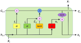
I implemented an LSTM in Java that can read a trained Keras models in order
to use it in some other Java projects. You can check the repository at [:Github:]

The ipython notebook exports the weights of an LSTM
and also exports some test for a random input sequence and the resulting output.
The Java implementation reads the exported weights and then applies them. All
matrix operations are implemented using jBlas.

  • The numeric helper class implements matrix loading and slicing.
  • Tanh and the sigmoid functions are also in the helper class.
  • The LSTM state is a separate class holding the cell state and the hidden activation.
  • The LSTM holds all the weights and applies them to sequences.

The basic slicing of the weights is implemented using the same weight
coding as Keras [:Github:]

        self.kernel_i = self.kernel[:, :self.units]
        self.kernel_f = self.kernel[:, self.units: self.units * 2]
        self.kernel_c = self.kernel[:, self.units * 2: self.units * 3]
        self.kernel_o = self.kernel[:, self.units * 3:]

        self.recurrent_kernel_i = self.recurrent_kernel[:, :self.units]
        self.recurrent_kernel_f = self.recurrent_kernel[:, self.units: self.units * 2]
        self.recurrent_kernel_c = self.recurrent_kernel[:, self.units * 2: self.units * 3]
        self.recurrent_kernel_o = self.recurrent_kernel[:, self.units * 3:]

        if self.use_bias:
            self.bias_i = self.bias[:self.units]
            self.bias_f = self.bias[self.units: self.units * 2]
            self.bias_c = self.bias[self.units * 2: self.units * 3]
            self.bias_o = self.bias[self.units * 3:]